Lab 3: Development of a Field Navigation Map

Introduction

For this lab we were given the task of developing a navigational map for the Priory, a plot of land owned by the university on the outskirts of Eau Claire that contains a building, forest, and elevation changes. The purpose of this lab is so that we can create a map containing enough information needed to successfully find a number of navigation points in the Priory area, much like an orienteering course, only instead of being given a map, we needed to make it ourselves.

The assignment included creating two maps, one using the Geographic Coordinate System (GCS) and the other the Universal Transverse Mercator (UTM) to help give an idea of which coordinate system is better suited for navigation. Both of these are known as the two major global coordinate systems. The UTM in its nature preserves the shape of a given area, allowing for nearly perfect accuracy in measurement of up to 1 meter, thus this projection is most often used for navigational purposes. In addition, this projection is divided up into 60 different vertical zones.

(Figure 1) UTM zones

The zone that was specifically picked for the site of the Priory was the UTM Zone 15N. As you can see in the map below, western Wisconsin fits into this zone, thus giving the most accurate navigation.

(Figure 2) US UTM Zones. Eau Claire, WI falls in the 15N zone, and was therefore the zone that was chosen for this lab.

GCS uses latitude and longitude to determine location and it uses the decimal degree system which is described using degrees, minutes, and seconds, which, unlike UTM, is not a basic unit of distance.

(Figure 3) GCS using latitude/longitude and degrees/minutes/seconds

In order to be able to use our map in the field without measuring tape or lasers, we conducted a pace count for ourselves to see how many steps it would take us to walk 100 meters. We measured this by using a laser which digitally calculated the distance from one end of the desired field to the other. We proceed to walk the 100 meters while counting every time your left foot hit the pavement; this was done one more time to ensure accuracy. My personal pace count for 100 meters is 72 steps.

Methods

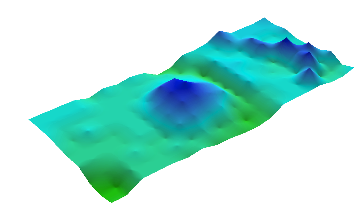
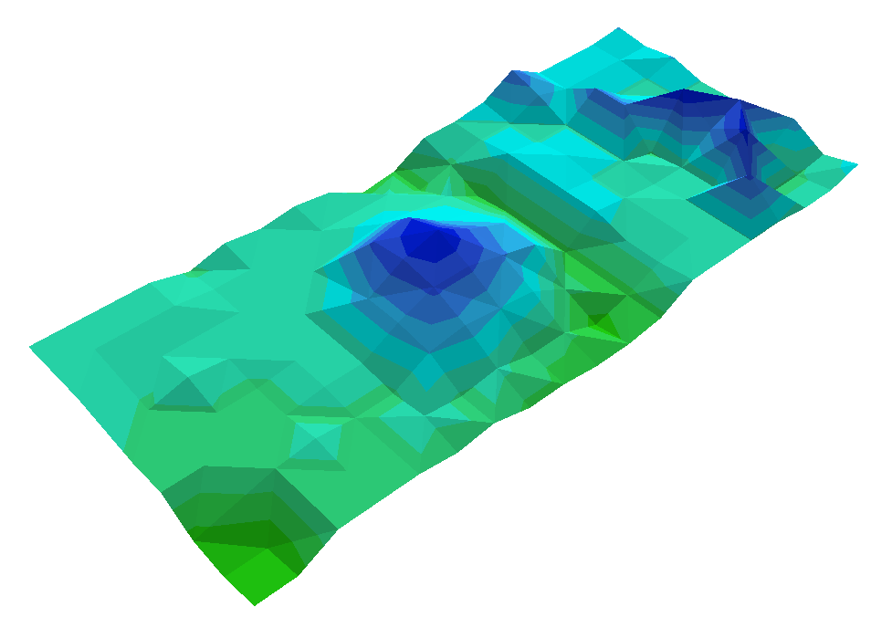
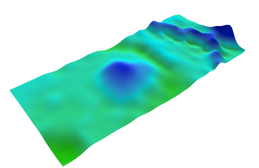
Within ArcMap, I was able to open the Priory Geodatabase that was given to us by Professor Hupy. This contained a number of files including imagery, 5 meter contour lines, 2 foot contour lines, DEM (digital elevation model), and the navigation boundary. The DEM allows for a nice and easy to understand visual using continuous data instead of the lines that are used to display the contour lines. From there I did a significant amount of playing around with the colors, and layers to appropriately display the maps. My objectives were to minimize clutter, yet provide maps that would help me discern the geographic locations in the field. Below are some of the individual files and their display image.


(Figure 4) 5 Meter Contour Lines. These were used on both maps (along with the elevation labels, seen on figures  8 and 9) because of their ability to portray elevation without coming across as too busy.

(Figure 5) 2 Foot Contour Lines. This file was not used in either map because of its clutter. The DEM was able to depict similar characteristics without all of the lines (see below).

(Figure 7) Gray Scale DEM. The darkest areas show the lowest elevation, and the lightest areas show the highest elevation.

On both maps I included the imagery to get a sense of relative location (e.g. east of the Priory building and half was down the east facing slope). I also wanted to include the 5 meter contour lines rather than the 2 foot ones, because the 2 foot contours were extremely close together which impaired the ability to see the imagery, DEM, and other features that I wanted to highlight (see figure 6).



(Figure 6) 5 Meter Contour Lines and 2 Foot Contour Lines. This display was avoided to reduce clutter on the map.

Using a scale bar in meters is vital to using the pace count that was established at the beginning of this lab. I chose smaller increments in order to be able to measure the distance during the actual navigation better. In addition, a grid system was used for both maps to improve the likelihood of accurate navigation. DEM and contour lines seemed to be an effective way to visualize elevation in both a static (contour lines) and dynamic (DEM) way.

For the GCS map, I wanted to focus on elevation change. The more darkly shaded areas depict lower elevation. One of the ideas I played around with was inverting the gray scale to show higher elevation in black. However that took away from more imagery than I was hoping for, even after changing the transparency.

(Figure 8) Coordinate System: NAD 1983 (2011)

 

In addition to the UTM coordinate system, I projected the image to Transverse Mercator. I chose this because UTM was based on this projection and it is widely used in mapping. Its angles are accurate everywhere, ensuring preserved direction. For this map I wanted to emphasize less elevation change  and more imagery in combination with the DEM. After the actual field aspect of this lab, I will have a better understanding of what works and what does not.

(Figure 9) Coordinate System: NAD 1983 UTM Zone 15N.
Projection: Transverse Mercator

On both of the maps, I left space outside of the navigation boundary to give a greater sense of the surrounding area. In case I get really lost and end up outside of the boundary, I will at least have a little leeway for error and can hopefully use the map to correct myself, that or cry for help!

Discussion

One of the concepts I found the most interesting was watching the shape of the navigation boundary change between the two different coordinate systems that I used. The GCS is more compressed and rectangular, whereas the UTM is a perfect square. I was thoroughly surprised at how challenging it is to include all of the components that you want to in a simple map. Overall I think in the field I will like the UTM map better, just because it appears that I will be able to glean more from it without analyzing it. Given that all of the data is the same and that only the GCS and projections are different, it will be interesting to see which one works better in the end for navigational purposes.

Seeing as I have not tested out my own map yet, I am rather curious to find out how the two maps vary in accuracy. When looking at the UTM zones, it was very evident that Eau Claire is right on the edge of zones 15N and 16N. I'm curious to know how much (or if) the location within the zone affects the accuracy of the navigational properties. Another issue that could arise in the future is the projection that I chose for the UTM. There could potentially be a better projection that I am unaware of using, thus making it more difficult to navigate in the field. I would like to spend more time analyzing the pros and cons of different coordinate systems and projections. If I need to make more navigation or preservation maps in the future I will be able to have a better handle on which projections to use.

Conclusion

I believe this lab will greatly help in future map creation. Normally when I have made a map I have not needed to worry about the map user implementing it for navigation purposes- it has normally served as a tool for visual geospatial description. Considering the coordinate system and projection for this type of map is vital in its accuracy and reliability. Another aspect of importance was the grid system. This tool will be important in the navigation process when we try to find the navigation points at the Priory in the future.

Considering that meters is the unit we used to create our 100 meter pacing, I am expecting the UTM to be easier to use in the field. However, there is always the issue with elevation change in that one often over or under compensates the pacing because of uneven terrain.

Lab 2: Visualizing and Refining the Terrain Survey

Introduction

This week we revisited the terrain survey that we had previously developed in the last lab. As a class we went back outside to our landscaped planters and evaluated each group's method. We found that we all did similar grid coordinate systems, but we all had various sized grids.

After evaluating our methods outside, we were to import our x,y, and z coordinates from Excel into an interpolation visualization in ArcMap. Interpolation allows a series of individual point to be developed into 'continuous' data using a measurement calculation to estimate the data (in this case elevation) in between the given points. This 2D image could then be imported into ArcScene, which is an ESRI extension that allows the user to view data in 3D. Seeing our points in 3D would then determine if we would need to back outside to take more measurements for our survey in order to make our 3D image more accurate.

Figure 1. Our plotted survey points after importing from Excel.

Methods

To import the Excel data into ArcMap, the points could not simply be imported into ArcMap as 'data', but 'x-y data', thus giving the points a spatial component. From here the tools in the 3D analyst (raster interpolation) were used. These tools included IDW, Natural Neighbors, Kriging, Spline, and TIN (a vector based tool that produces somewhat similar results to the raster interpolations). In ArcMap, the map can only be viewed in 2D, but after importing the data into ArcScene one can view it in 3D.

Figure 2. This image what the interpolation tools produce in ArcMap in 2D before importing the data into ArcScene.

These interpolation methods use different equations to develop the 3D image, meaning that one method would likely match the points given to make the interpolation look the most complete. For our group's data the 'Spline' interpolation looks the most appropriate. This is due to the smoothness of its edges and looking most accurate compared to the other methods. Here are the various methods in greater detail:

IDW is a 3D analyst tool that interpolates a raster surface from points using an inverse distance weighted technique.

IDW

Natural Neighbor is considered an "area-stealing" interpolation that finds the closest subset of input samples to a query point and applies weights to them based on proportionate areas to interpolate a value.

Natural Neighbor

Kriging differs in that it is a tool that assumes the distance or direction (in this case both) between sample points through a multistep process.

Kriging

TIN or triangulated irregular network database, is the only non-interpolation tool that was used. It also is the only vector based triangulation process used in this lab. It generally works better for a large number of points for a small area, such as an engineering project.

TIN

Spline is another interpolation tool that estimates values using a mathematical function that minimizes overall surface curvature, resulting in a smooth surface that passes exactly through the input points. This and IDW interpolation are consider deterministic interpolation methods. This is the method that we decided looked the best, thus we also used this tool in processing the second survey 3D imaging, pictured below.

Spline- Survey 1

Although 'spline' looked like it represented the landscapes well, there were still some issues with the 3D image that could only be fixed by going out in the field again to take more measurements. The error that we found the most profound was in the 'ridge' section of the planter. In relation to our 12 by 12 cm coordinate system, the ridge was not intended to fit the form of a grid, therefore its diagonal shape was missed in the measuring process. This likely could have been prevented using a smaller grid, but when looking at the other landforms in the 3D imaging, their lack of dramatic elevation change appeared fine in the final 3D shape.

We developed a new plan to cut our grid down from 12 by 12 cm to 12 by 6 cm so as to be more precise in the area of the ridge to define its dramatic elevation change. This second survey was only conducted on the last third or so of our survey area because the smaller elevation change of the other landforms did not appear to be necessarily re-surveyed. The same methods from the first survey were conducted to ensure accurate points comparatively to the second survey.

Figure 3. The portion of our planter that was re-surveyed with 6 cm increments is shown with the pink string. A singular string was moved in 12 cm increments vertically to this picture, similar to the first survey.

Figure 4. The ridge is shown that we wanted to resurvey. Measurements were taken for every other line of string because we had already measured half of those rows in the previous survey.

The number of '6' was developed because of it being the half way mark of our previous data, thus allowing us to mark '.5' intervals into Excel for our y-coordinates instead of having to develop a more difficult method of collaborating our existing data with the re-surveyed one.

Figure 5. Modified Excel data after increasing the number of survey points. Whereas our z data (column 3) is in cm, the x and y data (columns 1 and 2) are in unitless forms. To create the modified coordinate system, we chose 6 cm in order to be able to easily change some of the y coordinates into halves (thus .5 justifies the new points)

Once these points were taken, the same steps were repeated in taking the data from Excel, importing it into ArcMap, running the 3D interpolation tools, and importing it into ArcScene to evaluate its success comparatively to the first, less detailed survey.

Figure 6. Survey 2 with the x,y, and, z coordinates

It appeared that 'spline' also looked the best for the second survey set of data. However, there was one hill that was created in the making of the second spline that did not appear in the first one. This made me question if it was inaccurate measuring, or the fault of the mathematical equation for this particular interpolation method.

Spline- Survey 2

Discussion

In our class discussion, we found out that each group's coordinate system was based on a previous classes'  lab one decisions. I think by realizing this, we need to consider the broader picture instead of looking back on other blogs to serve as a basis for our projects. While the past projects might be good, there could, and probably are, better ideas if we take the time to channel them. In defense of the chosen grid coordinate system, this provided a quick and easy way to record data, where as a coordinate system without a grid would likely take longer to make due to individual measurements of the points, especially in the cold weather conditions.

We should have considered altering our testing methods the first time around when it came to the ridge, but we were set in thinking that the coordinate system had to be uniform in its measurement.

Looking back at our coordinate system, the second time we should have made it a 6 by 6 cm grid. There were still some errors in the final 3D interpolation of the second survey and it looks like we should have had more points to do such.

Working in ArcMap and ArcScene has been another test of my patience and ability to troubleshoot. However, the more I work with this program, the more I believe I have the ability to pick it apart and figure out why certain tools are not working. For example, an interpolation tool was showing up as an error for over an hour, when someone kindly pointed out that I had my ArcMap files within my geodatabase and that I was likely overloading it by having .jpg and .mxd files in it. It is the small details like that in which I am starting to be able to address and knowing that if all of the steps I am doing see to be right, it is probably due to a small knit picky error that does not even directly relate to the program.


Conclusion

Being able to take time to correct our errors and evaluate our decisions from lab one was invaluable. In most classes after I have finished a project, I always want to go back and revise it because I either learn how to make it better or I collaborate with others to gain more knowledge on the subject.

This lab provides for a good example of a real life situation in which the first trial run of a project does not suffice, so a second more improved version must be developed. In addition, this repetition allowed me to better understand how to use the program and become more proficient at using its features.

Having this lab gave a potential real world connection. In most jobs, taking each survey point would cost money, meaning that taking an exoboriant number of survey points would likely be over budget and not worth the cost. Taking too few means either leaving the output data as showing a poor visualization or yet again going into the field to take more points. This does not seem like an outright issue, but if that field you need to go to is half way around the world, you want to be able to get that survey right the first time. I have learned that it is of utmost importance to come up with a sufficient survey or research method before going out into the field. If our group had developed a better plan initially, we would not have needed to go back out into the freezing cold, and granted our stakes were not very high in this case, later down the road it is bound to be.