Lab 7: ArcPad Data Collection II

Introduction

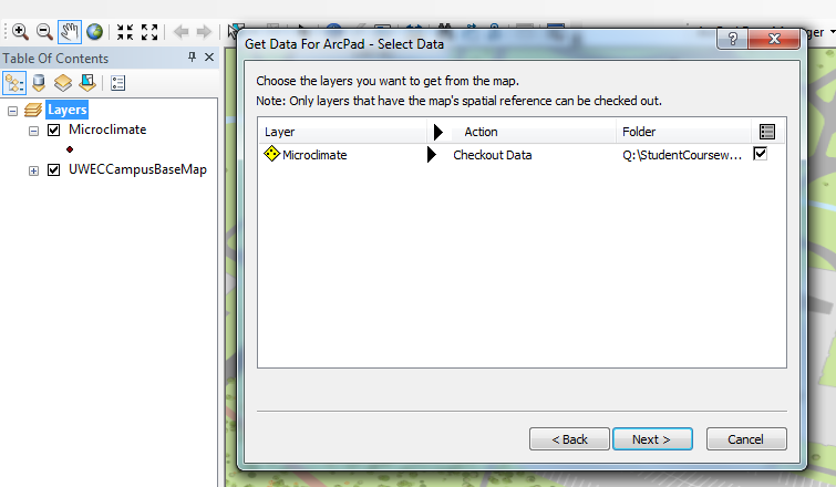
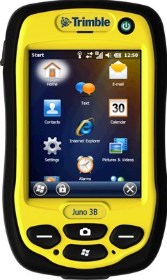
This week's lab was yet another continuation of the weeks prior. Last week consisted of testing out the microclimate geodatabase in the field, which then led to the understand of what worked and what did not. For lab this week, a refined geodatabase was created for the entire class (thanks to Zach Hilgendorf) in order to be able to go out into the field to collect data and bring it back into one ArcMap document. The purpose of this lab was to connect the past few week's knowledge and create the full microclimate data set for the entire campus by using the Trimble Juno GPS (see figure 1) to record the data in combination with the Kestrel weather meter (see figure 2).

Figure 1. This is the Trimble Juno GPS that was used in the data collection during this lab. It has the capabilities of an ArcPad application which allows for data collection directly into the mobile version of ArcMap.

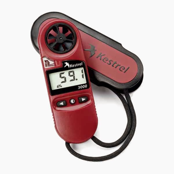Figure 2. This is the Kestrel 3000, which measured temperature (at the surface and 2 meters), wind speed, wind chill, dew point, and percent humidity for the microclimate data collection in this lab.

Methods

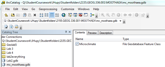
Before heading out into the field, it was vital that everyone was able to deploy the correct map and database onto their Juno to ensure that no mistakes were made. If errors were realized either in the field or once back in the lab, the entire data collection process would have to be redone to ensure accuracy.

The University of Wisconsin- Eau Claire campus is geographically distinctive in that it has a large hill (or more accurately a terrace) that divides lower campus from upper campus as seen in figure 3. Lower and upper are divided by the string of trees in the south west portion of the map. In addition, the Chippewa River runs along the north side of campus with a footbridge running over it for pedestrians to cross to get off campus or to the two academic buildings over the river.

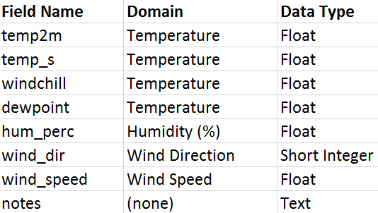
For the data collection, the same features were collected as for the last data collection: temperature at the surface, temperature at two meters, windchill, dewpoint, humidity (%), wind speed, ground cover, and notes. One feature was neglected, wind direction, because of lack of compasses for the class. The class was instructed to collected about 100 GPS points per groups of two and assigned a specific area on upper or lower campus to cover. One member of the group was in charge of using the Kestrel to determine the various climatic readings, while the other member inputted the data taken from the Kestrel to the Trimble Juno.

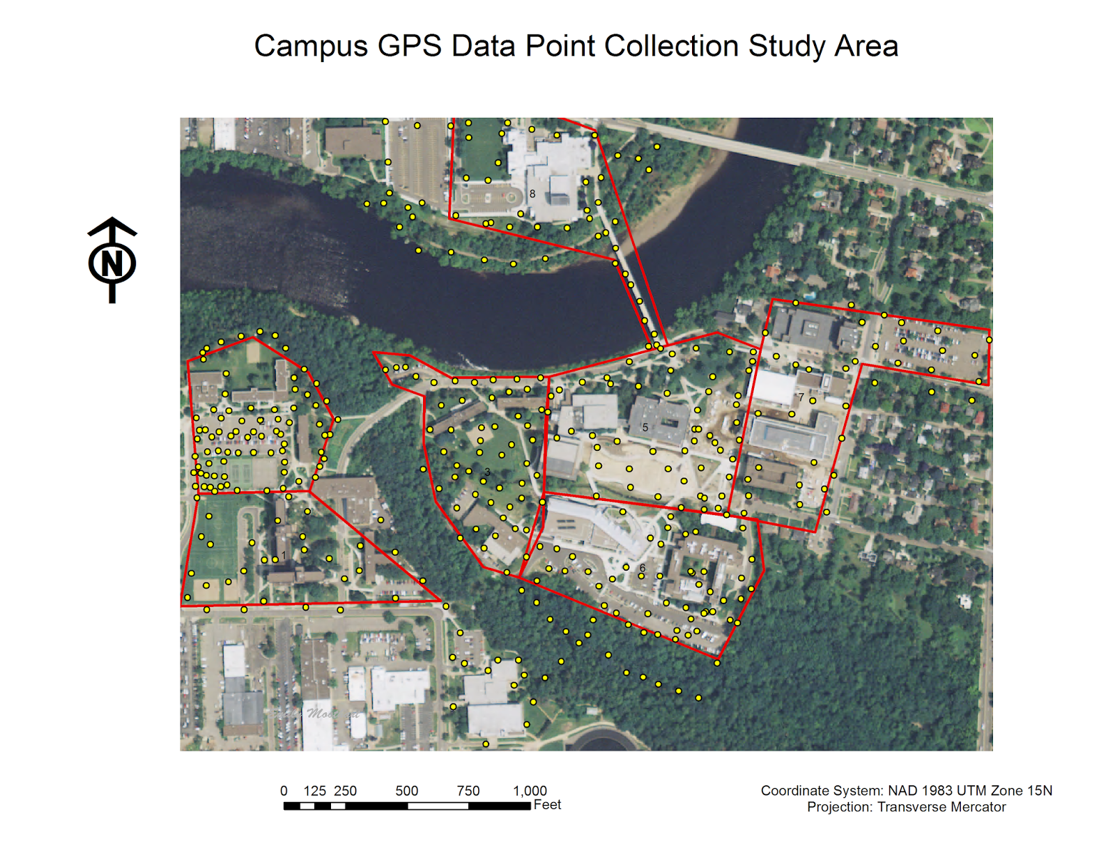Figure 3. Campus GPS Data Point Collection Study Area. This map depicts all of the points that were collected throughout lower campus (central portion of map) and upper campus (western portion of map). The red polygons indicate the data collection areas assigned to groups of two.

Once all of the data was collected by the class, the data was imported into a single feature class in one ArcMap file. This allowed the entire class to have access to each other's points in an editable form. In order to see continuous microclimate data for the campus, an inverse distance weighted (IDW) interpolation was performed. This interpolation technique was used for its ability to see local variation with a large number of sampling points.

Overall, the data showed a clear indication that Putnam Park (the heavily wooded region in the south west portion of the map) was cooler in temperature than the rest of the campus.

One weather measurement that was run was dew point (see figure 4). This is defined as the temperature at which the moisture in the air forms visible drop of water. This test was conducted in Fahrenheit.

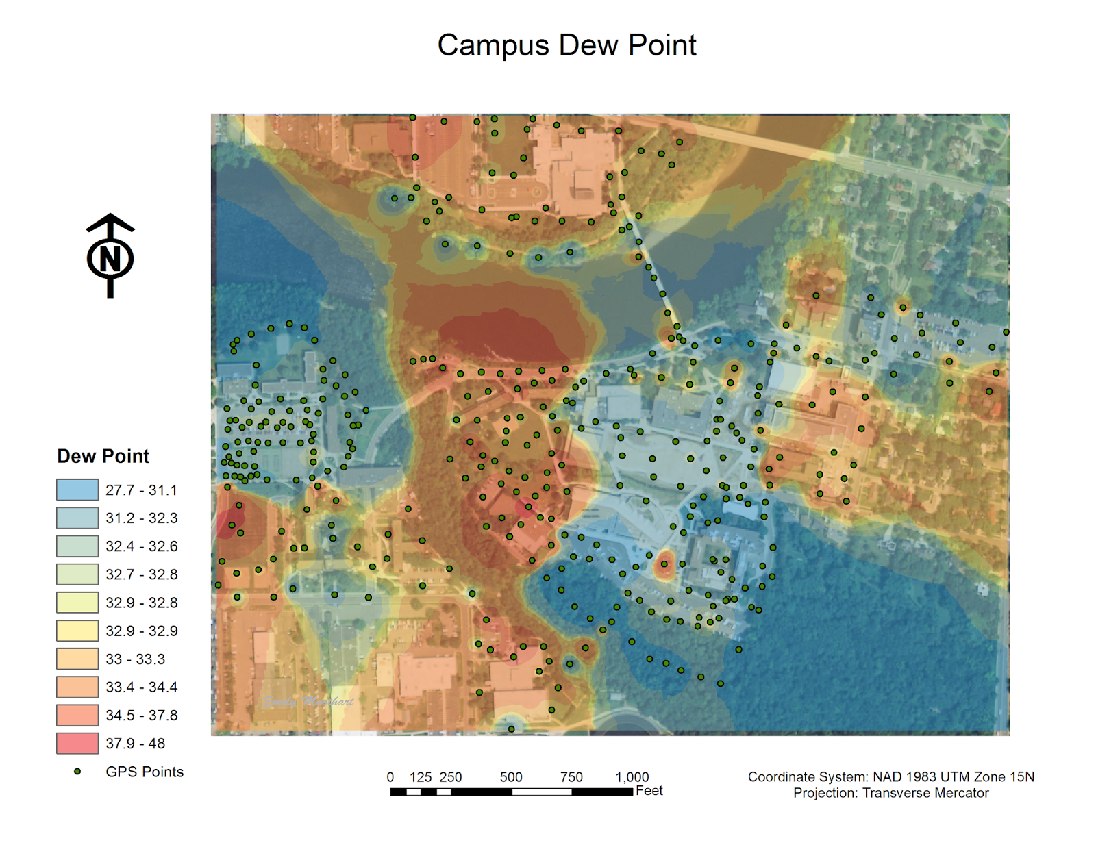Figure 4. Campus Dew Point (Fahrenheit). The regions that have higher dew point are generally areas around open water, or in the case of this particular day on campus, waterlogged because of the snow melting. The lowest dew point is located in the general area of the parking lots which contain a lot of cement, and likewise almost no water.

Relative humidity is another variable that was tested for the campus microclimate (see figure 5). It is defined as the ratio of partial pressure of water vapor to the equilibrium vapor pressure of water at the same temperature.

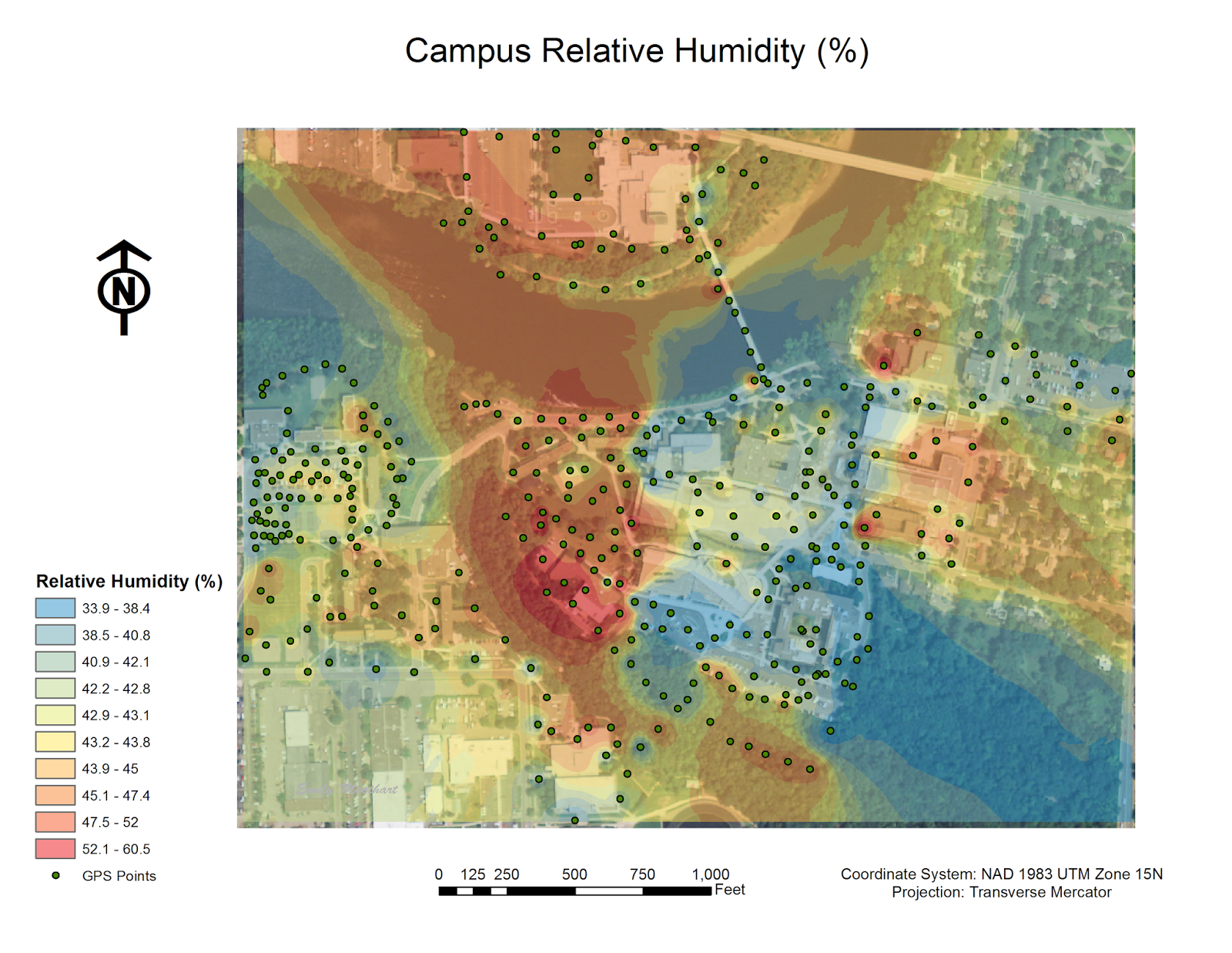Figure 5. Campus Relative Humidity. This map is almost identical to the dew point map above. The regions that have higher humidity are generally areas around open water, or in the case of this particular day on campus, waterlogged because of the snow melting. The lowest relative humidity is located in the general area of the parking lots which contain a lot of cement, and likewise almost no water.  

Temperature is an easy to understand concept that really aids in the initial understanding of a microclimate (see figure 6). Although at first it did not make sense that the yellow symbol was consuming the map, it was realized that the range of the symbology was between 0 and 60 degrees Fahrenheit. This is obviously an input error that effected the output of the map display.

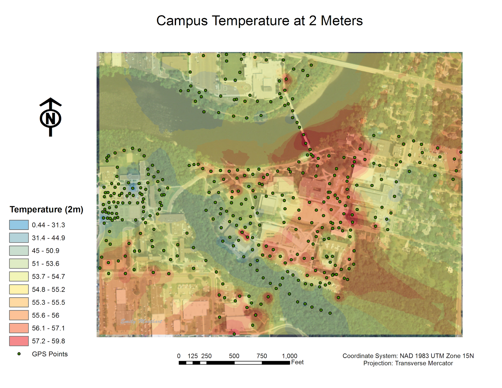Figure 6. Campus Temperature at 2 Meters (Fahrenheit). The coldest regions on the map are the ones located under tree cover. After analyzing the attribute table, it was realized that one of the groups neglected to include any two meter data. The 'null' area is shown in the middle of the red segment in the east-central portion of the map. With more data, there would have likely been more variation in interpolation output. 

Although temperature at the surface should be very similar to the temperature at two meters, it is still important to collect the data to compare the variation between the two temperature readings (see figure 7).

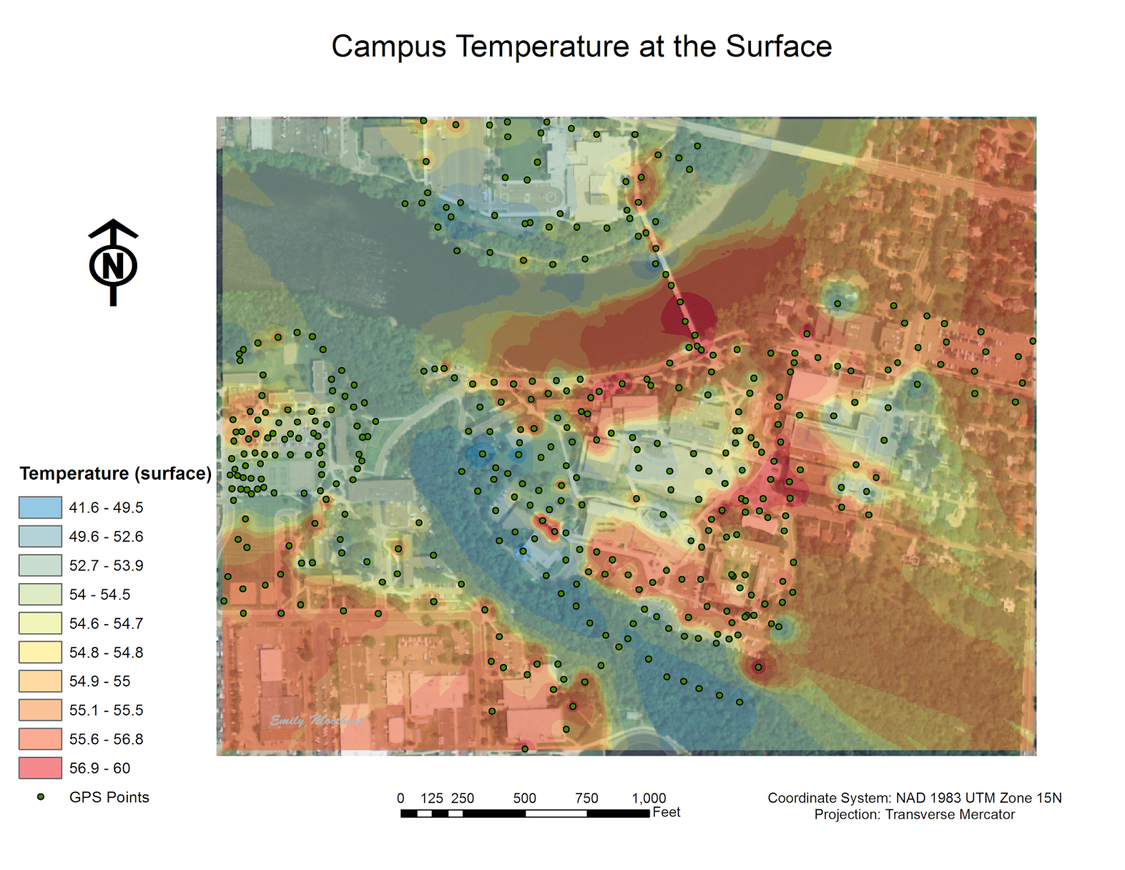Figure 7. Campus Temperature at the Surface (Fahrenheit). The coldest regions on the map are the ones located under tree cover. This is similar to the campus temperature at two meters.

Relatively high wind speed have an effect on this campus largely due to the Chippewa River running through it. Below is a map indicating the wind speeds, in miles per hour, throughout the campus (see figure 8).

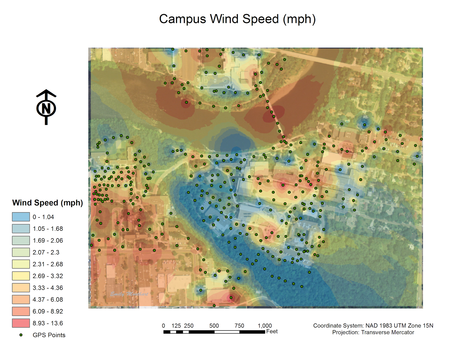Figure 8. Campus Wind Speed (miles per hour). There is a direct correlation to where the tree cover is and the wind speed. In Putnam part, there were no wind where there is the most tree cover. In addition, exposed areas along the river's shore have higher wind speeds.

Wind chill is another weather variable that was measured (see figure 9). Wind chill is the perceived decrease in air temperature felt by the body on exposed skin due to the flow of air. Wind chill is always lower than the air temperature when the formula is valid. The issue with using the Kestrel is that there are often readings of the wind chill that are higher than the temperature of the surface or at two meters, which is inaccurate.

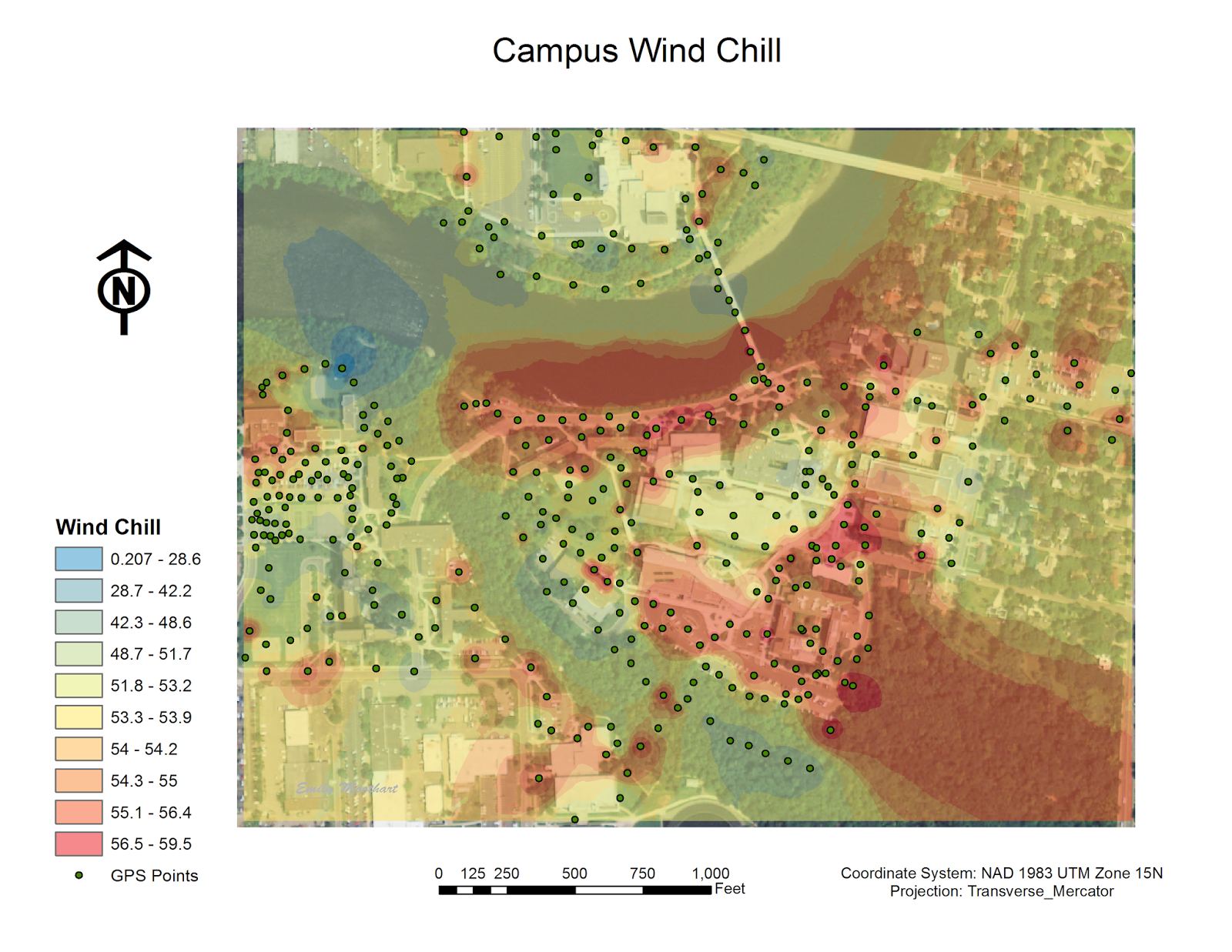Figure 9. Campus Wind Chill (Fahrenheit). Not surprisingly, the highest wind chill was along the river. It was surprising when analyzing the data that there was still fairly strong winds in parking lot behind the Davies Student Center (the lower central area indicated in red).

Ground cover is determined as the terrain type on a given surface such as grass, black top, snow, gravel, open water, sand, concrete, and other (such as woodchips). There were a couple of points in the data set that were missing the ground cover data, so those few points were determined as 'undefined' on the map below (see figure 10). Ground cover plays a potentially important role in the measurement of certain weather conditions. One of the more important measurements that would be variable due to this is temperature at two meters and temperature at the surface. If the day had been quite sunny the black top would have likely been much warmer at the surface than at two meters, which would have affected the outcome. According to the data collection records, there really is not much of a difference between the two temperature readings, so this factor does not seem to have played a role on the microclimate data taken on this particular day.

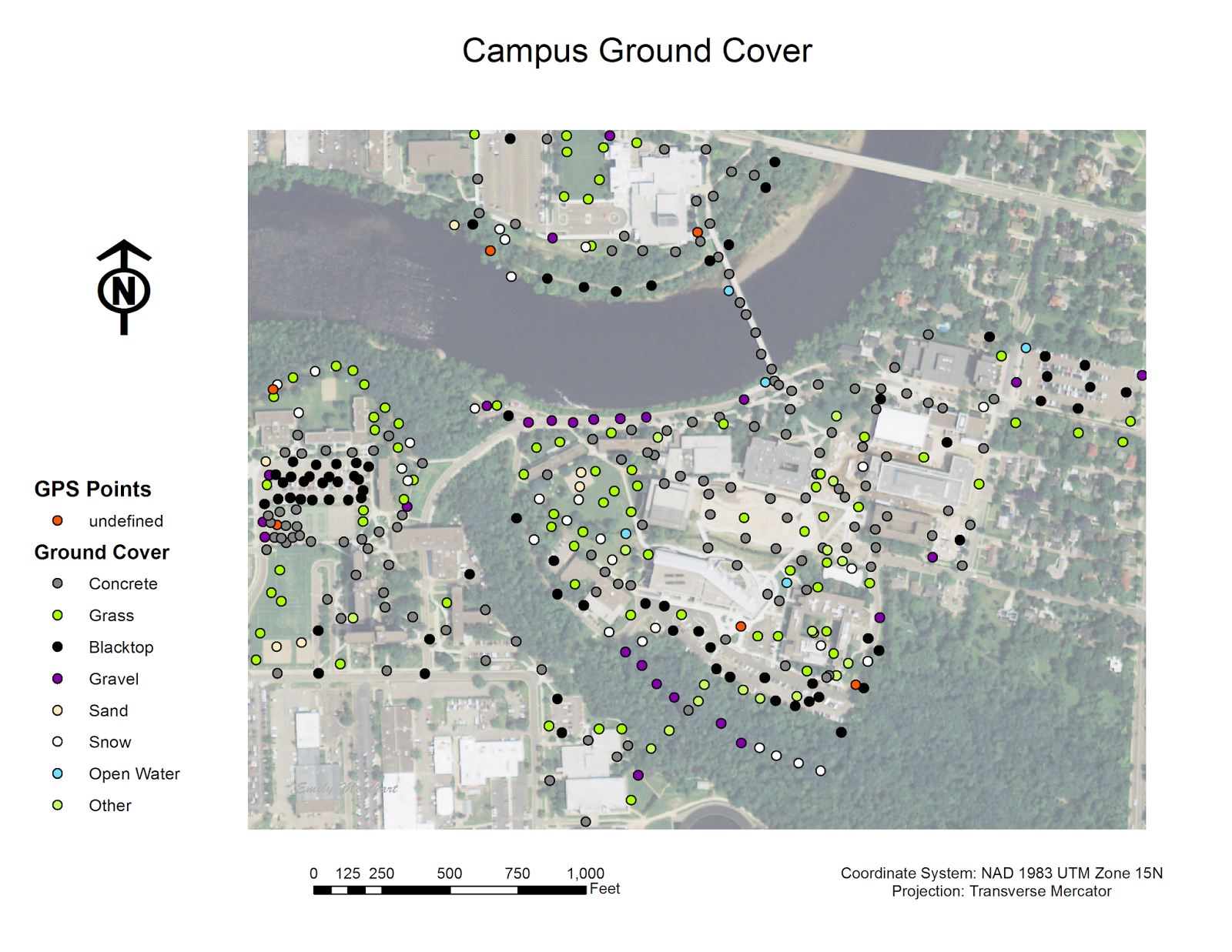Figure 10. Campus Ground Cover. This displays the variation in surface features in which the data was collected on.

Discussion

From the last geospatial data collection, the temperature outside increased about 30 degrees Fahrenheit. This shows that even if you believe the domain originally set will cover the likely temperatures for the time of year, think again. It is definitely better to have a larger sampling of GPS points; comparatively to last week's test run, this grouping of points allows for a much more detailed spatial analysis.

However, by looking in the attribute table for the data points, there were many errors when inputting the data. One error is that a group failed to measure the temperature at two meters for all of their designated region (see figure 11). Additionally, another group entered '0's into their temperature at two meters column (see figure 12). Both of these mistakes would therefore impact the visual outcome of the IDW interpolation that was performed.

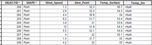Figure 11. As seen in the 'Temp_2m' column, there were no recorded measurements at two meters, which would have affected the interpolation output for the map.

Figure 12. An error was made in the data input of 'Temp_2m' in that '0' was entered, which is a clear outlier in the data. This would therefore skew the interpolation output and range for the data as a whole. 

Regarding the data collected, I was surprised that there was not more of a distinctive microclimate impression directly from the presence of the Chippewa River. There were regions along the river that indicted a similar microclimate, but I would have thought that it would have been more consistent along the river's shore.

In addition, after the three years of living on campus, I have realized that climbing up the stairs to get to the top of the hill next to the river generally has a drastic change in temperature and wind speed as one walks up. It would be intriguing next time the survey is done to take a point at every set of stairs to see the a possible change in climate.

Although we collected all of the points within a two hour period, there was still a lot of variability when it came to the weather readings, especially wind speed in a given minute. To me, this makes it very difficult to overall gather an accurate reading of the campus microclimate. In addition, the class failed to effectively use the notes field during the data collection out in the field. It would have been interesting to know other weather conditions that could have played a part in the outcome of the data.

Conclusion

This particular lab ran quite smoothly because of the attention to detail in the steps prior to the data collection. There would have been a much different discussion if we had been inefficient in deploying our database or if there had been a failure in the database. Due to human error, there are a few circumstances in which the data is incorrect, but as a whole, the microclimate lab was a success. That simply shows that one needs to take time when doing all portions of the lab, and that missing one step can effect the entire class's interpretation of the data.

I feel like after this lab I have a really good handle on how to create a reliable geodatabase and know how to confidently deploy it, collect the data, bring it into ArcMap, and analyze the data. This knowledge will help immensely in future geographical activities so that more attention can be given to the data analysis, not just the data collection. Having this course has really helped with gaining a solid understanding of how to use ArcMap in many applications that will be useful in the future.

Lab 6: ArcPad Data Collection I

Introduction

After creating the geodatabase for the campus microclimate study from the previous lab, it was time to take the geodatabase and put it to the test out in the field. This weeks' lab was to serve as a test run for the official data collection day, which will take place during the next lab. The goal was to figure out all of the short comings of our individual geodatabases and learn from that to create a class 'master' geodatabase in which to collect all of the official GPS points for next week. This required taking out the Trimble Juno GPS (see figure 1) to record the data in combination with the Kestrel weather meter (see figure 2) to gather the microclimate data.

Figure 1. This is the Trimble Juno GPS that was used in the data collection during this lab. It has the capabilities of an ArcPad application which allows for data collection directly into the mobile version of ArcMap.

Figure 2. This is the Kestrel 3000, which measured temperature (at the surface and 2 meters), wind speed, wind chill, dew point, and percent humidity for the microclimate data collection in this lab.

Methods

Some initial work had to be done before going out in the field. This included adding the 'microclimate' feature class as well as a recent campus basemap to ArcMap. The Juno GPS was then connected to the computer via USB to be able to export the ArcMap file to ArcPad (the mobile version of ArcMap). Then the 'ArcPad Data Manager' toolbar and its extension needed to be turned on to enable the data transfer to the Juno. There was an issue with using the basemap that was found on ArcGIS Online (UWECCampusBaseMap) (see figure 3). The 'Get Data From ArcPad' would only process the microclimate feature class, without the basemap (see figure 4). Therefore a different basemap (ortho_1-1_1n_s_wi035_2013_1.sid) was used and the 'Get Data for ArcPad' successfully transferred (see figure 5).

Figure 3. This is the error pop-up that occurred when attempting to use the 'UWECCAmpusBaseMap' basemap. The operation was successful when using the 'ortho_1-1_1n_s_wi035_2013_1.sid' basemap. 

Figure 4. This is the unsuccessful basemap and only the microclimate feature class could be exported from this. See below for successful export.

Figure 5. This is the successful basemap that included both the microclimate feature class as well as the basemap of the UW- Eau Claire campus.

After the basemap uploaded to the Juno, it was time to put the 'Microclimate' feature class to the test. Beside for the stylus being touchy and making it difficult to input the data, the collection went off without a hitch. Using the Kestrel weather meter was another story. The temperature reading moved quite slowly from the temperature inside the building to the temperature outside. It was difficult to know when the temperature was truly appropriate for outside.

Following the collection of points throughout campus, it was time to import the data from the Juno to ArcMap. During the initial attempt to import the data, an error occurred, which prevented the data from showing up in an editable format. Some trouble shooting occurred to attempt to resolve the issue, but the only way that was proven to work was to create a new .mxd and import the ArcPad data as well as the 'microclimate' feature class.

When opening up the attribute table for the 'microclimate' feature class, all of the points collected in the field were there, but they appeared twice, while indicating that there were ten points taken, not five (see figure 6). This is an issue that will need to be fixed before next weeks' official data collection.

Figure 6. The table shown is the attribute table from the points collected from this lab. Notice that points 6-10 are a repeat of  points 1-5. This was an error somewhere in the process of collecting the points in ArcPad and transferring the data to ArcMap. 

Discussion

There were quite a few things that went wrong in this lab, mostly before heading out in the field. The most troubling one that occurred for me was not being able to 'Select Data' for the UWECCampusBaseMap. This was solved, however, by using a different base map. In the field, I was mostly successful with my data collection, except that the 'groundcover' field was on a separate page than the rest of the fields, which confused me for a bit.

In addition, it was frustrating to collect the data because there would be times when the ArcPad data collection page would exit without being able to go back and edit the GPS points. This is why there are quite a few 'null' spots on the attribute table (see figure 7).

Figure 7. The table shown is the attribute table from the points collected from this lab. The null values are the points where I missed the collection.

I used two basemaps to compare how accurate the GPS points were. It was interesting because the precision of the points depended on what basemap was being used. The figure 8 basemap was the one that I used during the process of collecting the points in the field. However, according to where I actually stood, the online campus basemap (figure 9) was actually more accurate. This surprised me, but it is hard to compare two images of very different pixel quality.

Figure 8. This is the basemap imagery that was brought into the field and imported back into ArcMap. While the points are in the general region, there are a couple that should be on the cement, but appear to be on the grass. 

Below are a series of maps created from the five GPS points taken in the field. Figures 9 and 12 are individual points, but figures 10, 11, 13-15 are interpolation based to show the likely change in data spatially across the campus mall. A couple of maps are missing due to lack of data collected in the field including wind direction and temperature at surface.

Figure 9. This is a zoomed in image of the points taken on campus. The only point on this image that is 'off'' is the bottom right point which should be on concrete. Note that this imagery is slightly different than figure 8's.

Figure 10. Campus Percent Humitidy. The bottom right point was missed during this data collection. 

Figure 11. Campus Dewpoint.

Figure 12. Campus Ground Cover. The ground cover of the campus was not able to be interpolated because it was in the form of text, not short or long integer.

Figure 13. The wind chill point was missed in the bottom right, thus creating a much different visual than if the bottom right point had been included.

Figure 14. Campus Wind Speed.

Figure 15. Campus Temperature at 2 Meters. 

Conclusion

In Geographical Information Systems I, we did a similar GPS project, so it was great to bring back some of the tools I learned last year. It is really wonderful to be able to grow from skills I learned previously in GIS. For that project I created multiple feature classes, but for this one I was able to step it up a couple of notches and create multiple fields within one feature class.

As experienced in class, sometimes there are technical issues that can only be solved by trouble shooting, which can be rather frustrating at times. I have previously stated that this class is really helping me with patience, but that needs to be reiterated after this lab. If at first you don't succeed, try as many ways as you can, seems to be the solution.

Lab 5: Preparing a Geodatabase for Microclimate Field Collection

Introduction

As a class, Professor Hupy discussed the development of a geodatabase and its importance in developing a good geodatabase before heading out into the field. This lab was set up to prepare the class individually to be able to use ArcPad in the field to collect data on the micro climate of the campus. In order to properly collect the data, the class needed to have the background to effectively collect the data. This was especially important because the data will need to be collected in a short period of time so that time does not play a factor in understanding the campus micro climate. In addition, if one does not have all of the fields available when in the field, it will make it much more difficult for the user to manipulate the data once back in the lab. 

Part 1

In order to create a microclimate analysis, one needs to take the time to plan and prepare before going out into the field. This includes having the tools to do such. For this lab we will be using a Trimble Juno GPS (see figure 1). A single feature class will be created for the microclimate analysis. This is much simplier than having a feature class created for every attribute.  Data entry and analysis becomes much easier when the data is located under one feature class.

Figure 1. This is the Trimble Juno GPS that will be used in the data collection during this lab. It has the capabilities of an ArcPad application which allows for data collection directly in to the mobile version of ArcMap.

When developing a geodatabase, one must consider what various subcategories fall under the definition of a microclimate. A microclimate is considered a very small area that varies in temperature, humidity, and surface type to name a few factors.We will be considering temperature at the surface, temperature at two meters, windchill, dewpoint, humidity (%), wind direction, wind speed, ground cover, and notes. Having this variety of attributes will give us a solid understanding of the variation of the climate of the campus.

As mentioned later in the lab, setting appropriate domains before going out in the field is the make or break it point in having a successful field and data input experience. The above attributes require to be set up with their own domains to place limits on the data entered in the field. For example, having a range of -100 to 100 degree Fahrenheit for the temperature attribute does not make sense because Wisconsin in March rarely gets above 50 degrees. Therefore, setting a more realistic domain will minimize the likelihood for errors when manually entering the information into the Juno.

Part 2

Methods

Step 1- Construction of a Geodatabase

There is a great amount of planning that needs to occur on a desktop compter before one goes out into the field with a Trimble Juno equip with ArcMap. First go into ArcCatalog and create a file geodatabase by right clicking on the folder you would like to place the data in. This will be where your feature classes, with all of its fields, will be stored (see figure 2).

Figure 2. This is what one sees in ArcCatalog when accessing and creating their file geodatabase. This one is titled 'mc_moothaea.gdb'. 

Step 2- Development of Geodatabase Domains

This is where you will build your domains. Domains are the location in which one sets up the parameters for the data entry. From the domain, one can create the field name within a feature class. By integrating multiple fields within one feature class, the data can be viewed in a much more concise manner, and it is much easier to separate specific fields into layers rather than the other way around.

To edit domains, right click on your file geodatabase and click on 'properties'. The 'domain' tab is where the entry process will start. First, one will enter the name of the desired domain (as established in the pre-planning), and then create the description it. It is important to be thorough, because it may make sense to you, but it might not make sense to someone else in the future (see figure 2).

Figure 2. Here are the domains set for this lab. These are the aspects of the microclimate that were set up during the pre-planning process.

Step 3- Development of Domain Ranges

There are two domain types that one can create for their data. One is range, which allows the user to set restrictions on the data input capabilities. These domains are all using numerical quantities. The data for this lab was mostly in range form, which includes 'Humidity (%)', 'Temperature', 'Wind Direction', and 'Wind Speed'. The other type of domain is text. This allows you to enter sub-categories in the domain field type. The domain type in this lab that contains text is the 'Ground Cover' domain. The ground cover text is added in the 'coded values'. Here grass, snow, concrete, black top, open water, gravel, sand, and other codes are added all with their own separate descriptions (see figure 3).

Figure 3.This is the screen found after right clicking on the file geodatabase under 'Properties'. 

In addition, one must set the field type based on the domain type chosen. A domain type of range has a variety of field type options to choose from including short integer, long integer, float, and double. All have various numerical capabilities listed below (see figure 4).

Figure 4. This is a description of the data types that can be used for numerical domains. For this lab, short integer and float were the desired data types.  

The Excel document below gives an overall view of the domains and their parameters (see figure 5).

Figure 5. Data inputted into ArcCatalog. This is an Excel spreadsheet of what is all entered into the domains within the file geodatabase in figure ___.

Step 4- Construction of a Feature Class for Later Deployment to ArcPad

Creating a feature class is simple comparatively to the process of developing domains. To create a feature class, go into ArcCatalog, and right click on the file feature class that contains the domain information (mc_moothaea.gdb) (see figure 6). Then select 'new', 'create feature class' and set the name of the feature class, and coordinate system.

Figure 6. This is the contents of the 'mc_moothaea.gdb'. 'Microclimate' is the file geodatabase feature class that contains all of the domains and fields that are needed to go out into the field and record data.

Then begin the entry of the field name and its data type as seen below in figure 7.

Figure 7. This screen is found within the feature class properties which can be accessed by right clicking the file geodatabase feature class 'Microclimate' under the 'Fields' tab. Within this tab, one can set the field name that will appear in the attribute table. The domain for the individual fields is created here by setting the data type, which must match the domain's data type (e.g. float, text, short integer) that was developed during the domain's creation.

An important note is that the domain for the individual fields are created here by setting the data type, which must match the domain's data type (e.g. float, text, short integer) that was developed during the domain's creation. Through this process, the attributes are connected to the domains. The field name for the feature class differs from the field name of the domain type in that there can be multiple feature class field names that contain the same domain. For example, the 'temp_s', 'temp_2m', 'windchill', 'dewpoint', 'hum_perc' are all different feature class fields, but they have the same domain, temperature which is set to -30 -60. This means that none of these fields's input numbers can exceed -30-60. This is because they are all related to temperature and it would not make sense to have individual domains set up for each field type.This minimizes the likelihood of error in the data entry (see figure 8).

Figure 8. Each field name is a subcategory of the feature class 'Microclimate'. Each of the domains listed was originally developed in ArcCatalog and applied to the field names listed. Note that all of the fields involving temperature are all set under the 'Temperature' domain. This allows the temperature related field names to have the same domain, thus minimizing likely error.

Step 5- Importation of a Raster Background Data Set

A detailed base map is important to include for this lab so that when zoomed in, the imagery is not pixilated. This was found in the geospatial database found on the UWEC computers. This particular basemap is called City_Eau_Claire_3in_2013 (see figure 9).

Figure 9. This is what ArcMap looks like once the feature class and raster base map have been added. This is also the extent of the mapping region that will take place out in the field. 

Discussion

Some people in the class experienced different difficulties while creating their domains. By talking with these people about their issues, I feel that I will be able to prevent running into these issues later. One of the major issues that I ran into was not having one of my field names show up in the attribute table after creating the feature class. Professor Hupy was also having difficulties figuring out what I had done wrong, and so I decided to create a new .mxd file and re-import the feature class. After doing something this simple, all of the field names appeared. I learned that ArcMap can be very fussy and more often than not, there is either a slight error by the user, or just a glitch in the system. Patience is key to using ArcMap and already I have gained quite a bit of that in class.

We were also told to be very specific in creating a description of the domain. This was to ensure that if people were using our data in the future, that they would be able to understand the logistics of each of our domains to be able to replicate the domain or take our information and analyze its output. I know sometimes I struggle with explaining ideas effectively, but it is absolutely vital in order to collect data to be used for the future.

Conclusion

Developing a geodatabase can seem like a minimal task, but when it involves going out in the field and using the pre-determined domains and attributes, one does not want to miss a component. Taking time to think about the parameters and requirements prior to going out into the field will make the rest of the process much easier, even if it does seem to be a nuisance in the lab before going out into the field. 

Lab 4: Unmanned Aerial Systems Mission Planning

Introduction

Unmanned Aerial Systems (UAS) is a technology that the professor, Joe Hupy, knows quite a lot about. Because this is a quickly growing industry, he was eager to have us conduct a lab on the importance of mission planning for various projects and to learn the logistics of flying a simulator unmanned aerial vehicle (UAV).

For this lab, we were given the task of logging two hours on the simulator. Thirty minutes for four different platforms, or vehicles. Two of these had to be fixed wing and two had to be multi-rotor. A fixed wing is like a standard airplane, whereas a multi-rotor is more like a helicopter with multiple rotors (see figures 4 and 5). This variety was set to give the students an array of flying experience to determine which platforms should be used in future flight missions as well as getting a handle on flying them for the future UAV course offered next fall.

The UAVs typically have a computer programmed into them which serves as the 'auto pilot'. That being said, in no way should you rely on that to keep the UAV safe from harm. Endless issues could occur that would require the user of the remote to be needed including a change in wind conditions, computer programming error, unaccounted for trees or buildings, or a motor burning out. Typically, someone setting out on a UAV mission should have at least one other person with them, but it is best when there are three people in total: one to run the computer, another to serve as the remote user, and a third which serves as a spotter. In addition to the UAV's ability to be controlled by computer and remote control (see figure 1), a number of add ons can be attached to the vehicle. This includes, but is not limited to cameras, thermal imagery, remote sensing, and moisture sensors.

Figure 1. Remote controller for RealFlight flight simulator.

The flight simulator program (RealFlight 7.5) is designed to reduce the number of user/ environmental errors once out in the field.   The simulation allows the 'flier' to change various conditions (updrafts, wind speed) as well as the vehicle (anything from a blimp to a fighter jet) and flying location (a swamp, carnival, or flight school just to name a few). In addition, the flier can view the simulation in multiple modes such as on-flight, trailing (see figure 2), and ground view (see figure 3). While on-flight is the most fun, we were strongly encouraged to view it mostly in ground view, considering that none of us would ever experience actually flying on an unmanned vehicle.



Figure 2. A 'trailing' view in the RealFlight simulator.

Figure 3. Screenshot of the Aerial Field and its on screen virtual goggle view with the capabilities to see the angle and navigational direction of the UAV, and distance from the RC home base as well as the battery level.

There are a couple of main reasons why someone would want to use UAVs including its relatively small cost compared to a manned airplane or helicopter. In addition, because of its small size, it can get much closer to the desired location, thus giving a much higher resolution of imagery.

Methods

In order to get a bearing on the handling of the UAVs, the class needed to individually spend at least two hours using the flight simulator. In this time, a log was to be kept in order to get a better sense of how various vehicles operate in different conditions. In the log there were different sections which allowed the individual to look back and analyze how different conditions make it easier or more difficult to operate a vehicle. In addition, after the simulations were completed, the individual had a much better understanding of how the different platforms operated, which mission they would be the most successful in, as well as understand where their skill level was at for various platforms.

Two of the fixed wing UAVs were the Slinger and Yak-54 (see figure 4). The Slinger was a more difficult vehicle to run in my opinion because of its take off which seemed more temperamental due to the nature of manually having to angle it before launching it. If the start off was not solid, there was no easy way to correct it. The Yak-54 was easier in that it was more stable in the take off and while it was in the air. Because of the nature of the vehicle, it could travel at 70 miles per hour, which made it difficult to control closer to the ground without nose diving. However, when it was higher in the atmosphere, it was smooth sailing.

Figure 4. Fixed wing UAV, similar to the Yak-56 used in this lab.

The two multi-rotor UAVs that were flown were the Hexacopter 780 (6 motors) and the Octocopter 1000 (8 motors) (see figure 5). Both were quite easy to fly, but there were a couple of slight differences. The Octocopter did a lot better in windy conditions than the Hexacopter, but it was more difficult to move the Octocopter around. The Hexacopter would be better in tight fitting spaces with low wind conditions, say a more rural setting, whereas the Octocopter would be better in an open field. For both of these UAVs, the reason for crashing was that the battery died. The Octocopter seemed to last longer (17 minutes airtime) whereas the Hexacopter only lasted 13 minutes. This was surprising because the battery life should be shorter on a UAV with more rotors. This could be potentially due to different weather or platform conditions.

Figure 5. Multi-rotor UAV. The two multi-rotor UAVs that were used in this lab were the Octocopter and Hexacopter. 

Here is the flight log that recorded the flight logistics for all of the platforms (see figure 6).

Figure 6. Flight log.

In addition to using the flight simulator, the class was given the task of building off the knowledge received in the simulation by applying it to two flight mission scenarios. The response to these scenarios were to be written as if the audience was the client. Here is one of the missions:

' A power line company spends lots of money on a helicopter company monitoring and fixing problems on their line. One of the biggest costs is the helicopter having to fly up to these things just to see if there is a problem with the tower. Another issue is the cost of just figuring how to get the things from the closest airport'

Dear Client: As was brought up in your concern with using a manned helicopter, it is difficult and costly to figure out the logistics of using a vehicle of that size. By utilizing a UAV, the need to use an airport to launch the vehicle would be eliminated. In addition, because the UAV is much smaller and unmanned, it is quite versatile and it will be significantly cheaper than using a helicopter. In order to keep the power lines, tower, and UAV safe, it is recommended that you use a multi-rotor vehicle due to its capability to hover and thus take detailed pictures of the tower. So you are aware, the more rotors there are on a UAV, the shorter the time it can stay charged, but according to your description, a greater lift from the rotors will provide you with a UAV that can take off very close to the site. In addition, more check ups on the tower can be utilized with the UAV because of the much lower cost in operation, thus allowing a higher customer satisfaction in the ability for the power lines to be working at a higher rate of success.

To be able to fully utilize the capabilities of the UAV for your project, I suggest using an ultraviolet (UV) detector, which would be able to detect the inconsistencies and wiring issues on your tower system. IHS Engineering 360 has what you are looking for, and here is more information regarding its uses and benefits.

This is scenario number two: 'A pineapple plantation has about 8000 acres, and they want you to give them an idea of where they have vegetation that is not healthy, as well as help them out with when might be a good time to harvest.'

Dear Client: Unlike using a manned helicopter to do the imaging for your field, a UAV would be able to provide you with high quality photographs and GPS coordinates that would allow you to see the when harvesting would be appropriate. Because UAVs are inherently cheaper to fly than a manned vehicle, you could fly a UAV more often to benefit the health of the crops as well as be able to monitor their growth. For your needs, I would use a fixed wing vehicle that would allow for long flight times (about an hour) as well as an easy ability to fly in a straight pattern to accurately cover your entire field.

Here is a scholarly report about Rice Crop Monitoring with Unmanned Helicopter Remote Sensing Images. This will give you an idea of how to read remote sensing data for your field. AIRSAR (Airborne Synthetic Aperture Radar) would be a good option to measure biomass of your pineapples. The Gimbal, which is a support that allows for angle rotation of on-flight devices, would be perfect for viewing the field with multiple angles, thus giving a better idea of crop conditions (see figure 7).

Figure 7. Gimbal attached to a DSLR camera which allows the camera's angle to be mechanically changed during flight.  

In addition, using an NDVI, or Normalized Difference Vegetation Index, will provide imagery which will easily determine the health of the pineapples (see figure 8).

Figure 8. NDVI imagery of fields. The green is healthy vegetation, yellow is dry or dormant plants, and brown is plowed fields or bare ground. This imagery would give a detailed view of the moisture content of the plants. 

Discussion

If I were to use more time for using the flight simulator I would definitely use it on the fixed wing vehicles. I found that they could be taken much easier windy conditions, and unlike the multi-rotor, it is much harder to stabilize for longer periods of time. However, using the simulator with the multi-rotor made it somewhat difficult to detect where the camera was facing from the ground level. I believe with more practice, this will get easier.

During the simulations, there was often an obstructed view of the UAV due to buildings, trees and land forms, and the sheer distance that was often between the ground view and the vehicle. This all played a part in the success of each flight. Most often I kept the view in ground mode to replicate a real life situation, but sometimes it was necessary to put the simulator in first person mode to track where the UAV was. A big help was the virtual goggle view that showed the direction of 'home', and its distance, as well as a few other helpful pieces of information (see figure 3). This setting was vital when using the Hexacopter 780 because the 60 mile per hour winds carried away the UAV without any hope of bringing it back.

The flying styles between the multi-rotor and the fixed wing UAVs were difficult to get used to. Whereas the multi-rotor UAV could be held steady by basically using the pitch (right joystick)(see Figure 1), the fixed wing's pitch joystick had to be flicked downward in order to stay in flight.

Conclusion

At the start of this lab, I had absolutely no idea of how UAS worked in the slightest. On the day that we had a trial run in class to test it out, I failed miserably at keeping the UAV in the air for more than 30 seconds. Since having two hours of flight under my belt I really feel like I have more of a handle on it. I realized that multi-rotor UAVs are much easier for me to control, yet they are better for covering smaller areas with a need for hovering abilities. I am really glad to have had this lab to better understand this up and coming technology that allows better and cheaper mapping of a multitude of scenarios.